

In the previous article we started learning some important stuff about Pandas, this great library of Data Science. From the creation of DataFrames to the description and alteration of them, a lot of topics were covered. But Pandas is not done - not by a long shot. In this article we will continue with several functions of Pandas that may not be so well known, but are certainly useful.
Grouping and Counting
We are going to continue with the wine dataset that we used in the previous article. There, it is explained how to load it, as well as the basics. This time, however, we are going to study our dataset. Let’s say we want to know how many unique wines we have.
We can do:
df.Wine.unique()
array([1, 2, 3], dtype=int64)
There are three different wines.
But how many registers we have of each?
We can group by the Wine column in the DataFrame:
df.groupby('Wine').Wine.count()
Wine
1    59
2    71
3    48
Name: Wine, dtype: int64
What is going on here? With the groupby function we can select a set of columns (or just one) by which to group the DataFrame.
We got what is called a DataFrameGroupBy object.
It has the same columns as the original DataFrame, but now grouped.
And with these groups, we can perform operations such as count, min, or even apply lambda functions:
df.groupby('Wine').apply(lambda df: df.loc[df.Alcohol == df.Alcohol.max()])
          Wine  Alcohol  Malic.acid   Ash   Acl  Mg  ...  Nonflavanoid.phenols  Proanth  Color.int   Hue    OD  Proline
Wine                                                 ...
1    8       1    14.83        1.64  2.17  14.0  97  ...                  0.29     1.98       5.20  1.08  2.85     1045
2    71      2    13.86        1.51  2.67  25.0  86  ...                  0.21     1.87       3.38  1.36  3.16      410
3    158     3    14.34        1.68  2.70  25.0  98  ...                  0.53     2.70      13.00  0.57  1.96      660

[3 rows x 14 columns]
A very long line, but let’s break it down.
It groups by wine, that is clear.
And we apply a lambda to the resulting DataFrame.
It will take the register where Alcohol is maximum for each of the wines.
And this just opens endless possibilities, such as the .agg() function.
.agg()
What is this function?
We have shown that we can group by elements and apply functions.
But sometimes, when we want to perform an analysis we want a lot of data.
And this is where .agg() comes in.
Instead of calling the functions one by one, we can aggregate all the data we want:
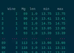
wine_mg = df.groupby(['Wine','Mg']).Alcohol.agg([len, min, max])
          len    min    max
Wine Mg
1    89   1.0  13.75  13.75
     90   1.0  13.41  13.41
     91   1.0  14.75  14.75
     92   1.0  13.05  13.05
     93   1.0  13.39  13.39
...       ...    ...    ...
3    113  1.0  13.08  13.08
     116  1.0  13.11  13.11
     120  2.0  13.17  13.27
     122  1.0  12.86  12.86
     123  1.0  13.50  13.50

[94 rows x 3 columns]
What we have done is grouping first by Wine and then by Mg, and getting the length, the maximum and the minimum.
Depending on the DataFrame, we can do more or less complex groupings, such as grouping by country and region.
And this DataFrame ties in with the next topic perfectly.
Multi-index
The keen eyed will have noticed an important difference in this new DataFrame with respect to the ones we have been working with: it is using a Multi-index.
This means that it is indexed by two different values.
Usually, this grants a fine granularity for a more sophisticated analysis.
When you have high dimensionality, or a hierarchical set of values, this can be a very interesting tool.
In this tutorial, we are going to see the basics of indexing, and how to return to a simple index.
Given that for a lot of applications it will be easier to convert a Multi-index to a regular indexed DataFrame and use the methods you already know.
The Multi-index is hierarchical, which means that it is ordered. This way, if you do:
wine_mg.loc[1]
     len    min    max
Mg
89   1.0  13.75  13.75
90   1.0  13.41  13.41
91   1.0  14.75  14.75
...  ...  ...    ...
127  1.0  14.23  14.23
128  1.0  14.22  14.22
132  1.0  13.76  13.76
You get the DataFrame where Wine is 1, with the single remaining index.
You can manipulate that new DataFrame to get specific values, or you can do:
wine_mg.loc[(1,95):(1,100)]
          len    min    max
Wine Mg
1    95   2.0  12.85  14.12
     96   3.0  13.50  14.39
     97   1.0  14.83  14.83
     98   3.0  13.05  13.86
     100  2.0  13.20  13.48
To get the values that go from Wine == 1 and Mg == 95 to Wine == 1 and Mg == 100.
Indexing with multiple indices can get complicated very quickly and it depends on each analysis if it is the proper tool. In case you want to go back to single indices, you can just do:
wine_mg.reset_index()
   Wine   Mg  len    min    max
0      1   89  1.0  13.75  13.75
1      1   90  1.0  13.41  13.41
2      1   91  1.0  14.75  14.75
3      1   92  1.0  13.05  13.05
4      1   93  1.0  13.39  13.39
..   ...  ...  ...    ...    ...
89     3  113  1.0  13.08  13.08
90     3  116  1.0  13.11  13.11
91     3  120  2.0  13.17  13.27
92     3  122  1.0  12.86  12.86
93     3  123  1.0  13.50  13.50

[94 rows x 5 columns]
That way, Wine and Mg are independent columns and you can use the methods explained previously. That way, you decide how to work your data.
Sorting
Finally in this section, we are going to see how to sort the data.
It is fairly simple: just calling the function sort_values:
wine_mg.sort_values(by='len')
          len    min    max
Wine Mg
1    89   1.0  13.75  13.75
3    122  1.0  12.86  12.86
2    96   1.0  11.45  11.45
     99   1.0  12.67  12.67
     100  1.0  12.64  12.64
...       ...    ...    ...
3    96   4.0  12.20  14.13
2    85   5.0  11.03  13.05
1    101  5.0  13.16  13.90
2    88   9.0  11.41  12.60
     86   9.0  11.82  13.86

[94 rows x 3 columns]
You just have to set the column (again, or columns) by which you want to sort and that’s it.
Take note of the parameter ascending to have an ascending or descending sorting.
Combining DataFrames
In this section, we are going to see how to combine several related DataFrames for their study. First, let’s divide our DataFrame:
 df_one = df.loc[df.Wine == 1]
 df_two = df.loc[df.Wine == 2]
 df_three = df.loc[df.Wine == 3]
Now, there are two main methods of combining DataFrames. The first is to put one just underneath the other. Let’s say we have two DataFrames of the same thing but obtained at different dates and we want to put them together to have one big DataFrame:
df_one_two = pd.concat([df_one, df_two])
     Wine  Alcohol  Malic.acid   Ash   Acl  ...  Proanth  Color.int   Hue    OD  Proline
0       1    14.23        1.71  2.43  15.6  ...     2.29       5.64  1.04  3.92     1065
1       1    13.20        1.78  2.14  11.2  ...     1.28       4.38  1.05  3.40     1050
2       1    13.16        2.36  2.67  18.6  ...     2.81       5.68  1.03  3.17     1185
3       1    14.37        1.95  2.50  16.8  ...     2.18       7.80  0.86  3.45     1480
4       1    13.24        2.59  2.87  21.0  ...     1.82       4.32  1.04  2.93      735
..    ...      ...         ...   ...   ...  ...      ...        ...   ...   ...      ...
125     2    12.07        2.16  2.17  21.0  ...     1.35       2.76  0.86  3.28      378
126     2    12.43        1.53  2.29  21.5  ...     1.77       3.94  0.69  2.84      352
127     2    11.79        2.13  2.78  28.5  ...     1.76       3.00  0.97  2.44      466
128     2    12.37        1.63  2.30  24.5  ...     1.90       2.12  0.89  2.78      342
129     2    12.04        4.30  2.38  22.0  ...     1.35       2.60  0.79  2.57      580

[130 rows x 14 columns]
The .concat() function from Pandas takes an array of DataFrames and pastes them together.
The columns named the same will combine, while the columns with different names will be created anew; and the DataFrame without said column will be filled with NaN.
If, on the contrary, we want to compare both DataFrames, we can use the join function.
That function will take two DataFrames with the same index and join them together.
Let’s say we want to get all the registries joined by the same value of Mg.
We do the following:
left = df_one.set_index(['Mg'])
right = df_two.set_index(['Mg'])
mg_join = left.join(right, lsuffix='_one', rsuffix='_two')
     Wine_one  Alcohol_one  Malic.acid_one  Ash_one  Acl_one  Phenols_one  Flavanoids_one  ...  Flavanoids_two  Nonflavanoid.phenols_two  Proanth_two  Color.int_two  Hue_two  OD_two  Proline_two
Mg                                                                                         ...
89          1        13.75            1.73     2.41     16.0         2.60            2.76  ...             NaN                       NaN          NaN            NaN      NaN     NaN          NaN
90          1        13.41            3.84     2.12     18.8         2.45            2.68  ...            1.69                      0.43         1.56           2.45     1.33    2.26        495.0
90          1        13.41            3.84     2.12     18.8         2.45            2.68  ...            1.84                      0.66         1.42           2.70     0.86    3.30        315.0
91          1        14.75            1.73     2.39     11.4         3.10            3.69  ...             NaN                       NaN          NaN            NaN      NaN     NaN          NaN
92          1        13.05            1.73     2.04     12.4         2.72            3.27  ...            2.04                      0.39         2.08           2.70     0.86    3.02        312.0
..        ...          ...             ...      ...      ...          ...             ...  ...             ...                       ...          ...            ...      ...     ...          ...
124         1        13.05            2.05     3.22     25.0         2.63            2.68  ...             NaN                       NaN          NaN            NaN      NaN     NaN          NaN
126         1        14.06            1.63     2.28     16.0         3.00            3.17  ...             NaN                       NaN          NaN            NaN      NaN     NaN          NaN
127         1        14.23            1.71     2.43     15.6         2.80            3.06  ...             NaN                       NaN          NaN            NaN      NaN     NaN          NaN
128         1        14.22            3.99     2.51     13.2         3.00            3.04  ...             NaN                       NaN          NaN            NaN      NaN     NaN          NaN
132         1        13.76            1.53     2.70     19.5         2.95            2.74  ...             NaN                       NaN          NaN            NaN      NaN     NaN          NaN

[84 rows x 26 columns]
The values with the same Mg will appear as one row, and the rest will have NaN in the corresponding fields.
Pipelines and Method Chaining
The last part of this tutorial will be a way to create pipelines. All these methods can be applied step by step, but they can also be applied together or one after another automatically. This is particularly useful when wanting to do the same processing to several similar DataFrames, or when you want to create a clean structure to understand later what is the process.
Let’s say we want to get a random sample of the Ash of those elements with the same Mg value, but without the NaN.
We can do:
(mg_join
    .dropna()
    .sample(5)
    [['Ash_one', 'Ash_two']])
     Ash_one  Ash_two
Mg
101     2.67     2.40
97      2.17     1.70
92      2.04     1.94
94      2.60     2.70
112     2.70     2.23
Chaining methods like this can create a simple and readable way to perform multiple operations to a DataFrame.
``.assign()`
With .assign(), you can modify or create columns inline.
To create a column called Ash_Greater_Two we can do:
mg_join.assign(
    Ash_Greater_Two=mg_join.apply(lambda df: df.Ash_one > 2, axis='columns')
    )
     Wine_one  Alcohol_one  Malic.acid_one  Ash_one  ...  Hue_two  OD_two  Proline_two  Ash_Greater_Two
Mg                                                   ...
89          1        13.75            1.73     2.41  ...      NaN     NaN          NaN             True
90          1        13.41            3.84     2.12  ...     1.33    2.26        495.0             True
90          1        13.41            3.84     2.12  ...     0.86    3.30        315.0             True
91          1        14.75            1.73     2.39  ...      NaN     NaN          NaN             True
92          1        13.05            1.73     2.04  ...     0.86    3.02        312.0             True
..        ...          ...             ...      ...  ...      ...     ...          ...              ...
124         1        13.05            2.05     3.22  ...      NaN     NaN          NaN             True
126         1        14.06            1.63     2.28  ...      NaN     NaN          NaN             True
127         1        14.23            1.71     2.43  ...      NaN     NaN          NaN             True
128         1        14.22            3.99     2.51  ...      NaN     NaN          NaN             True
132         1        13.76            1.53     2.70  ...      NaN     NaN          NaN             True

[84 rows x 27 columns]
.pipe()
Finally, the method .pipe() allows for a modification of the whole DataFrame inline, given a passed function.
This is a very specific function that can lead to interesting results, when needed.
In our case let’s say we want to remove all the NaN from the DataFrame.
We do the following:
mg_join.pipe(lambda df: df.dropna())
     Wine_one  Alcohol_one  Malic.acid_one  Ash_one  ...  Color.int_two  Hue_two  OD_two  Proline_two
Mg                                                   ...
90          1        13.41            3.84     2.12  ...           2.45    1.330    2.26        495.0
90          1        13.41            3.84     2.12  ...           2.70    0.860    3.30        315.0
92          1        13.05            1.73     2.04  ...           2.70    0.860    3.02        312.0
...         ...      ...              ...      ...   ...           ...     ...      ...         ...
110         1        13.51            1.80     2.65  ...           3.17    1.020    1.93        750.0
110         1        13.28            1.64     2.84  ...           3.17    1.020    1.93        750.0
112         1        14.20            1.76     2.45  ...           2.65    0.960    2.52        500.0
112         1        13.63            1.81     2.70  ...           2.65    0.960    2.52        500.0

[59 rows x 26 columns]
This function is a not-so-well-known one, but there are specific pipelines that can greatly benefit from it, when the modification of a DataFrame is very complex and needs a multiline function. Or sometimes, just the clarity of a short lambda can be decisive to choose this method. Anyway, now it is also in your toolbox.
Conclusion
In this second part of the tutorial, we have seen more obscure Pandas function. They are not usually seen in regular tutorials because the use-cases are more limited; but that can also be seen as more specific tools for more fine-grained jobs. With this, you have now the ability to process the dataset of your project with the proper functions, and to reach the goals writing clean and concise code that does what it needs to do.