

A trip through pandas
The moment we start in Data Science with Python, a name in the horizon appears: pandas. This is one of the best known libraries for data processing, and it is very well integrated in most of the machine learning frameworks such as scikit-learn or XGBoost. This is why it is almost essential to learn how to treat your data in Python with this library, and in this article we are going to go through some of the most useful things you can do with it.
Creating or Importing DataFrames
The first element you will need to know is the DataFrame, the structure where all data will be stored. This will be a database-like element that we will use and modify throughout the tutorial.
Note that the DataFrame is a complex structure that works for machine learning. If you are looking for Big Data, where you might have gigabytes and gigabytes of data and you might profit from cloud scalability; there are other more suitable libraries, such as Dask.
First things first, we need to import the library:
import pandas as pd
It is a well established convention to use the pd alias for pandas - plus you are going to be writing it so many times that it’ll be easier the shorter it is.
Now, the general rule for building a DataFrame is to do it as follows:
df = pd.DataFrame([[1,2,3],
                   [4,5,6])
Usually you are not going to be creating your datasets, rather, you will import them from somewhere.
In this tutorial, we are going to use the wine dataset found
here.
CSV files are widely used in machine learning to load datasets.
To load it:
df = pd.read_csv('./wine.csv')
To check that it loaded properly, let’s check the first five elements with:
df.head(5)
   Wine  Alcohol  Malic.acid   Ash   Acl   Mg  ...  Nonflavanoid.phenols  Proanth  Color.int   Hue    OD  Proline
0     1    14.23        1.71  2.43  15.6  127  ...                  0.28     2.29       5.64  1.04  3.92     1065
1     1    13.20        1.78  2.14  11.2  100  ...                  0.26     1.28       4.38  1.05  3.40     1050
2     1    13.16        2.36  2.67  18.6  101  ...                  0.30     2.81       5.68  1.03  3.17     1185
3     1    14.37        1.95  2.50  16.8  113  ...                  0.24     2.18       7.80  0.86  3.45     1480
4     1    13.24        2.59  2.87  21.0  118  ...                  0.39     1.82       4.32  1.04  2.93      735
We can see that it loaded even the name of the columns.
The read_csv function always takes the first row as the column name.
If you don’t want that to happen (because the columns name is not in the file, for example), you have to add header=None.
If you have a list of columns (must be unique), you can pass it with names=my_list_of_cols.
Finally, if your CSV has a different delimiter than a comma, let’s say a semicolon, you can specify it with sep=';'. With these options, you will pretty much load any dataset you have in your hands, and you are ready to go.
Indexing
Now that we have a set of data, let’s see how to pick parts of it for further study.
We already know how to take the first n elements, but what if we want to do a random sampling?
Of course, we do:
df.sample(5)
     Wine  Alcohol  Malic.acid   Ash   Acl   Mg  ...  Nonflavanoid.phenols  Proanth  Color.int   Hue    OD  Proline
79      2    12.70        3.87  2.40  23.0  101  ...                  0.43     1.95       2.57  1.19  3.13      463
135     3    12.60        2.46  2.20  18.5   94  ...                  0.63     0.94       7.10  0.73  1.58      695
164     3    13.78        2.76  2.30  22.0   90  ...                  0.41     1.03       9.58  0.70  1.68      615
144     3    12.25        3.88  2.20  18.5  112  ...                  0.29     1.14       8.21  0.65  2.00      855
133     3    12.70        3.55  2.36  21.5  106  ...                  0.17     0.84       5.00  0.78  1.29      600

[5 rows x 14 columns]
This can be very useful to extract graphs or to see the distribution of the data. But let’s say you want to be in control, and you need the registers 5 to 15.
You then have to use:
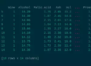
df.iloc[5:15]
    Wine  Alcohol  Malic.acid   Ash   Acl  ...  Proanth  Color.int   Hue    OD  Proline
5      1    14.20        1.76  2.45  15.2  ...     1.97       6.75  1.05  2.85     1450
6      1    14.39        1.87  2.45  14.6  ...     1.98       5.25  1.02  3.58     1290
7      1    14.06        2.15  2.61  17.6  ...     1.25       5.05  1.06  3.58     1295
8      1    14.83        1.64  2.17  14.0  ...     1.98       5.20  1.08  2.85     1045
9      1    13.86        1.35  2.27  16.0  ...     1.85       7.22  1.01  3.55     1045
10     1    14.10        2.16  2.30  18.0  ...     2.38       5.75  1.25  3.17     1510
11     1    14.12        1.48  2.32  16.8  ...     1.57       5.00  1.17  2.82     1280
12     1    13.75        1.73  2.41  16.0  ...     1.81       5.60  1.15  2.90     1320
13     1    14.75        1.73  2.39  11.4  ...     2.81       5.40  1.25  2.73     1150
14     1    14.38        1.87  2.38  12.0  ...     2.96       7.50  1.20  3.00     1547

[10 rows x 14 columns]
But what if you want to know just the Alcohol and Ash of those registers?
Then you need:
df.loc[5:14,['Alcohol', 'Ash']]
    Alcohol   Ash
5     14.20  2.45
6     14.39  2.45
7     14.06  2.61
8     14.83  2.17
9     13.86  2.27
10    14.10  2.30
11    14.12  2.32
12    13.75  2.41
13    14.75  2.39
14    14.38  2.38
Whoa, some changes here.
Why? The first change is to replace iloc by loc.
This is fairly simple.
While iloc works with indices, loc works with labels.
If we want to select a column by its name, we need the label; but if we had the number we could still use iloc.
Second is the range.
Before we used 5:15 but now 5:14? This is because iloc uses the standard ranges in Python, excluding the last one.
But given that loc works with all datatypes, including strings, it is more convenient to include the last one.
If you wanted to look for an alphabetical value from a to s it is easier to write a:s than a:t (knowing that t goes after s).
And complexity increases when it is full words we are using.
The only caveat is to take it into account when indexing with integers.
Lastly, there is a list of values.
Even if it is only one value (Alcohol), it needs to be a list.
Now, let’s say we want to be even more accurate.
We want to know from those registers which ones have Alcohol greater than 14:
df.loc[5:14,['Alcohol', 'Ash']].loc[df.Alcohol > 14]
    Alcohol   Ash
5     14.20  2.45
6     14.39  2.45
7     14.06  2.61
8     14.83  2.17
10    14.10  2.30
11    14.12  2.32
13    14.75  2.39
14    14.38  2.38
We can chain different loc operations to filter the DataFrame even further. And see that df.Alcohol?
Yes, we can access the columns of the DataFrame as if they were attributes of an object.
Let’s make it more complex, and filter also when Ash is smaller than 2.4:
df.loc[5:14,['Alcohol', 'Ash']].loc[(df.Alcohol > 14) & (df.Ash < 2.4)]
    Alcohol   Ash
8     14.83  2.17
10    14.10  2.30
11    14.12  2.32
13    14.75  2.39
14    14.38  2.38
We can see that loc uses binary objects to make the comparisons, that’s why we use the & as a binary operator and not && as a logic operator.
If we wanted to specify an “or” operator, we would use a single pipe |.
Creating new values
When processing the data to study the relationships, or to train a model, there are lots of times when creating new data is needed. Sometimes you need to build a value from existing values, or to split a certain value in two. Sometimes you have a string that represents multiple values and you want to encode them. Or other times you just think you might have seen an interesting ratio and you want to check how some values behave together.
Let’s say you want to have a new value that represents the ratio Alcohol to Ash.
It is as simple as write the following:
df['AlcoholAshRatio'] = df['Alcohol'] / df['Ash']
df.head(5)
   Wine  Alcohol  Malic.acid   Ash   Acl   Mg  Phenols  Flavanoids  Nonflavanoid.phenols  Proanth  Color.int   Hue    OD  Proline  AlcoholAshRatio
0     1    14.23        1.71  2.43  15.6  127     2.80        3.06                  0.28     2.29       5.64  1.04  3.92     1065         5.855967
1     1    13.20        1.78  2.14  11.2  100     2.65        2.76                  0.26     1.28       4.38  1.05  3.40     1050         6.168224
2     1    13.16        2.36  2.67  18.6  101     2.80        3.24                  0.30     2.81       5.68  1.03  3.17     1185         4.928839
3     1    14.37        1.95  2.50  16.8  113     3.85        3.49                  0.24     2.18       7.80  0.86  3.45     1480         5.748000
4     1    13.24        2.59  2.87  21.0  118     2.80        2.69                  0.39     1.82       4.32  1.04  2.93      735         4.613240
Here we have our ratio, to use it to plot a graph, to pass it to a model, etc. But instead of having to look at all the values to see how that ratio behaves, we can just study the most important data related to it with the following command:
df.AlcoholAshRatio.describe()
count    178.000000
mean       5.562817
std        0.693379
min        3.578947
25%        5.107217
50%        5.561649
75%        5.991097
max        9.095588
Name: AlcoholAshRatio, dtype: float64
Well, we have that our new value has a very low standard deviation, and that its percentiles are close to one another. Except from some outliers (as shown by the max and min values), it seems that indeed Alcohol and Ash are related. This could be an important information, depending on what we do with the data.
Declarative Programming
We have seen how to create values from other columns, but we can go even further beyond, with the power of declarative programming.
.map()
The first element we are going to use will be a map.
For those who don’t have yet the grasp of declarative programming, a map is a function that takes a set of values and “maps” them to a second set of values.
This is done by using a lambda function.
Let’s say we want to invert the AlcoholAshRatio column.
We can just do:
df.AlcoholAshRatio.map(lambda p: 1/p)
0      0.170766
1      0.162121
2      0.202888
3      0.173974
4      0.216767
         ...
173    0.178702
174    0.185075
175    0.170309
176    0.179954
177    0.193914
Name: AlcoholAshRatio, Length: 178, dtype: float64
Now we can see it as a ratio from 0 to 1. Maybe easier to plot or to study. But… wait. Have we lost the original ratio?
df.AlcoholAshRatio
0      5.855967
1      6.168224
2      4.928839
3      5.748000
4      4.613240
         ...
173    5.595918
174    5.403226
175    5.871681
176    5.556962
177    5.156934
Name: AlcoholAshRatio, Length: 178, dtype: float64
No.
As we can see, the original ratio is not modified.
These functions won’t modify the original value.
Which is specially useful to build even more new columns:
df['AshAlcoholRatio'] = df.AlcoholAshRatio.map(lambda p: 1/p)
   Wine  Alcohol  Malic.acid   Ash   Acl   Mg  Phenols  Flavanoids  Nonflavanoid.phenols  Proanth  Color.int   Hue    OD  Proline  AlcoholAshRatio  AshAlcoholRatio
0     1    14.23        1.71  2.43  15.6  127     2.80        3.06                  0.28     2.29       5.64  1.04  3.92     1065         5.855967         0.170766
1     1    13.20        1.78  2.14  11.2  100     2.65        2.76                  0.26     1.28       4.38  1.05  3.40     1050         6.168224         0.162121
2     1    13.16        2.36  2.67  18.6  101     2.80        3.24                  0.30     2.81       5.68  1.03  3.17     1185         4.928839         0.202888
3     1    14.37        1.95  2.50  16.8  113     3.85        3.49                  0.24     2.18       7.80  0.86  3.45     1480         5.748000         0.173974
4     1    13.24        2.59  2.87  21.0  118     2.80        2.69                  0.39     1.82       4.32  1.04  2.93      735         4.613240         0.216767
.apply()
Say now that we want to transform the whole DataFrame by applying a function per row.
We want to create a new value that checks if AlcoholAshRatio is an outlier, and divide it in low or high outlier; or in medium value.
We can do a function such as this:
 def AAR_outlier(row):
     aar_mean = df.AlcoholAshRatio.mean()
     aar_std = df.AlcoholAshRatio.std()
     if row.AlcoholAshRatio > aar_mean + aar_std:
         row['AAR_outlier'] = 'high'
     elif row.AlcoholAshRatio < aar_mean + aar_std:
         row['AAR_outlier'] = 'low'
     else:
         row['AAR_outlier'] = 'mid'
     return row
df.apply(AAR_outlier, axis='columns')
    Wine  Alcohol  Malic.acid   Ash   Acl     Mg  Phenols  Flavanoids  Nonflavanoid.phenols  Proanth  Color.int   Hue    OD  Proline  AlcoholAshRatio  AshAlcoholRatio AAR_outlier
0     1.0    14.23        1.71  2.43  15.6  127.0     2.80        3.06                  0.28     2.29       5.64  1.04  3.92   1065.0         5.855967         0.170766         low
1     1.0    13.20        1.78  2.14  11.2  100.0     2.65        2.76                  0.26     1.28       4.38  1.05  3.40   1050.0         6.168224         0.162121         low
2     1.0    13.16        2.36  2.67  18.6  101.0     2.80        3.24                  0.30     2.81       5.68  1.03  3.17   1185.0         4.928839         0.202888         low
3     1.0    14.37        1.95  2.50  16.8  113.0     3.85        3.49                  0.24     2.18       7.80  0.86  3.45   1480.0         5.748000         0.173974         low
4     1.0    13.24        2.59  2.87  21.0  118.0     2.80        2.69                  0.39     1.82       4.32  1.04  2.93    735.0         4.613240         0.216767         low
..    ...      ...         ...   ...   ...    ...      ...         ...                   ...      ...        ...   ...   ...      ...              ...              ...         ...
173   3.0    13.71        5.65  2.45  20.5   95.0     1.68        0.61                  0.52     1.06       7.70  0.64  1.74    740.0         5.595918         0.178702         low
174   3.0    13.40        3.91  2.48  23.0  102.0     1.80        0.75                  0.43     1.41       7.30  0.70  1.56    750.0         5.403226         0.185075         low
175   3.0    13.27        4.28  2.26  20.0  120.0     1.59        0.69                  0.43     1.35      10.20  0.59  1.56    835.0         5.871681         0.170309         low
176   3.0    13.17        2.59  2.37  20.0  120.0     1.65        0.68                  0.53     1.46       9.30  0.60  1.62    840.0         5.556962         0.179954         low
177   3.0    14.13        4.10  2.74  24.5   96.0     2.05        0.76                  0.56     1.35       9.20  0.61  1.60    560.0         5.156934         0.193914         low

[178 rows x 17 columns]
Just as before, it did not modify the original DataFrame.
Note that to apply it row-wise, we added the parameter index=columns.
This might seem counter-intuitive, so be careful when applying the functions.
Instead, index=rows means that the parameter passed to the function will be a column.
Lastly, the keen-eyed might have noted that this is just a more complex way of what we did to create the AlcoholAshRatio before.
Indeed, a DataFrame supports a set of basic operations to transform its columns, such as addition, multiplication, etc. These operations are much more efficient and faster, but much more limited in complexity.
It is the good programmer who knows the tools at hand and when to use them to create an efficient and powerful pipeline, in the end.
Sometimes you will need the speed of a simple sum between two columns, other times you will need the expressivness of a function that is applied per row (or column) despite it being slower.
pandas gives you both tools, and it is up to you to choose wisely.
Closure… or not?
pandas is a truly marvel when it comes to data treatment and study. It allows to do a huge deal with the data, when you know how to handle, and it is one of the most multi-purpose tools you can have in your data scientist toolbox. In this tutorial, we have but scratched what a DataFrame can do; and even with this, a great deal of data treatment can be done.
In a second part, we will explore more aspects of pandas, such as how to group columns, or do SQL-like queries. How to sort by different indices, or how to split and join multiple similar (or not so similar) datasets. How to build a transforming pipeline that can process similar DataFrames. We are not done yet.