

Know your allies
One of the best known libraries when it comes to machine learning tools in Python is Scikit-Learn. This very efficient, open source, commercially usable library contains a ton of different resources to carry out most of the machine learning projects you have in mind. Moreover, its great compatibility with most other Python libraries in the area make it awesome if you just need a specific part of its functioning and want to integrate it with other more state-of-the-art algorithms. You can install it just like any other Python library:
pip install scikit-learn
First things first: our data
The first thing we are going to do is fetch our data. Scikit provides with several toy datasets and several more complex ones. For this tutorial, we are going to use a real world dataset. This means that it will be more difficult to get a good prediction, and also that some computing times might take longer depending on your computer, so be wary of that!
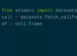
from sklearn import datasets
cali = datasets.fetch_california_housing(as_frame=True)
df = cali.frame
The dataset we are going to use is a regression set that contains some California housing information. It was obtained from here, and its target is the median house value for California districts.
It is a regression dataset, which means that the objective is to generate a floating point number, not to give a determined classification. When loading it, we are using the DataFrame version of the set, and we can manipulate it as we explained previously.
Preparing our data
The first thing we are going to need is to separate it in target and data.
Most of the machine learning algorithms take those two distinctive parameters, so we are going to define the set of columns and slice the DataFrame accordingly.
Upon reading the DataFrame definition from the Scikit webpage (or studying it with df.head()) we know the last column is the target, therefore:
data_cols = df.columns[:-1]
target_col = df.columns[-1]
X = df[data_cols]
y = df[target_col]
Easy approach to scoring
The easiest way to test how an algorithm is working is dividing the dataset in training and test splits. This means training your model with a part of the data and checking its accuracy with other. Though not the best validation strategy, it is often one of the most used to quickly check the performance of some algorithm. For that, Scikit offers a great tool:
from sklearn.model_selection import train_test_split
X_train, X_test, y_train, y_test = train_test_split(X, y, test_size=0.33, random_state=42)
This divides our dataset in a train split two thirds of our original set and the remaining third in a test split. Oftentimes you will see this approach used twice, with train, dev and test. You will iterate with train datasets and validating them against the dev dataset, to avoid overfitting against your test dataset. For this tutorial, we will keep it simple, as the focus is on the library and not the complete, strict machine learning procedure.
Choosing our regressor
AdaBoost, KNeighbors, MLP… There are a huge number of regressors in Scikit. They have one approach to which one to choose here. However, you can decide based on your previous experience or gut sometimes. In fact, all of them have the same methods, so anyone you choose will work exactly as described here - in fact many other libraries have the same methods to be “plug and play” with Scikit.
For this tutorial, we are going to use a Random Forest classifier. In order to import it:
from sklearn.ensemble import RandomForestRegressor
tree = RandomForestRegressor(random_state=0, n_jobs=-1)
Scikit has differentiated both regressors and classifiers, so be sure to import the proper algorithm. Now we have to pass it the data and see how well it performs:
tree.fit(X_train, y_train)
tree.score(X_test, y_test)
0.8042411820492733
Depending on your CPU, the algorithm will take longer or shorter.
See that n_jobs=-1 up there? That is telling Python to use all the available cores when training.
In heavily multithreaded process, such as Ensemble Models training, a high core count CPU can really speed up the process.
For other hardware, though, such as GPU acceleration for Neural Networks it might be better to use other libraries that support it.
What if we want to be more rigurous?
We said before that a train test split was the quick dirty way, but is there a better way to judge the performance of our algorithm? One of the better approaches is called cross validation. This means that we divide the dataset in folds, and we train with all of them but one and test against that one. We do that testing once per fold, so that we have a better global idea. To be even more accurate, we can do those folds stratified, this is, with a similar number of registers per class for every fold. And for all of this, Scikit offers us a great tool:
from sklearn.model_selection import cross_validate
cv_results = cross_validate(tree, X, y, n_jobs=-1)
{'fit_time': array([2.23339105, 2.34541059, 1.89533162, 2.32840872, 1.88032889]),
 'score_time': array([0.05301046, 0.02300501, 0.05300927, 0.02150393, 0.03050542]),
 'test_score': array([0.53493929, 0.70331888, 0.74232084, 0.62710629, 0.68075127])}
What we have here is that cross_validate will automatically stratify the dataset in 5 folds by default.
Again, this task can be paralelized, which is tipically a good idea.
Here , we can see that the test score of our algorithm is not so good as we thought, and that the previous good result might be due to some lucky train test random split.
Now is where the machine learning process starts, tweaking hyperparameters, modifying the dataset, etc.
Now it’s your turn!
Bonus
There are three important elements we have not talked about because they can very well be part of their own tutorial, but you should experiment on your own if they fit your working process:
Encoders
All the datasets provided by Scikit have integers or floats, but never strings on their columns. Why? Because its algorithms and functions work exclusively with numbers. But as we know, the real world has all kinds of data that cannot be just represented with numbers. To convert them, we have the Encoders, elements that can create a correlation between a specific string to a specific integer. Really useful as a preprocess for your data.
Search
We have talked before about hyperparameters. They are the little nuances in the models that can lead to wildly different results. Things like the maximum depth of a tree, the number of neurons in a CNN or the kernel in a SVM can be crucial to the result of the model. And there are ways to automate the trial and error process of fine-tuning them. GridSearch does an exhaustive search through all the specified parameters, while RandomSearch does a random, limited search in a range of parameters. Each have their uses, so feel free to experiment.
Pipelines
Just as we mentioned in the Pandas tutorial, there are some times that your whole process needs several steps.
Perhaps it needs to encode some data and make some transformations before training your model.
And perhaps that is dependent on the folds of the cross validation, so you need to do it all per each fold.
That is where
Pipelines come into play.
You can define the pipelines with all classes and methods who have a fit and a transform method, and a final classifier (or regressor) who has a fit method.
They can be really useful for a complex data science process.
Conclusion
Scikit is a huge, well used library that helps in every part of the machine learning process with its comprehensive functions and classes. In this tutorial we have seen the most typical use case, but Scikit is much more than this. Don’t hesitate in exploring its different classes to look for the ones that are the best fit for you.