Peeking Inside the Black Box: Explaining Artificial Intelligence models

A Brief Introduction

We live in the age of data and new technologies. More and more, Artificial Intelligence is coming to our lives, from the image processing after a picture is shot in our phones to the recommendation algorithm in most content places. And the number of companies that want to introduce some AI process to their workflow increases by the minute.

Soon, AI systems will be diagnosing illnesses, granting mortgages, etc. But then doubts arise. A lot of those AI systems will be black box systems, most likely Neural Networks or Ensembles. Basically a lot of automatic learned equations and parameters that are going to tell everybody if they are fit to buy a house, or if they have this or that illness.
But can we really trust these systems? They have been proven wrong in the past, showing incredible and unexpected biases.

Here is why the trend is moving towards making AI fair and understandable. There are great initiatives like fast.ai that focus on unbiased AI, but here we are going to use some of the latest framework to explain existing models.
Whether you have an AI pipeline in your company or you are learning how to use the latest Neural Network models, this tutorial will explain you a bit more about what is going on inside that process.

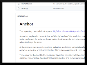
Anchor

There are plenty of papers researching XAI (eXplainable Artificial Intelligence), but there are not so many frameworks that can currently take an existing model and explain its internal processes. This kind of post-hoc explanation is very interesting because it does not have to reimplement and retrain the existing pipelines, but rather can work as a new addition to those pipelines.

In this article we will explain Anchor, a state-of-the-art library programmed in Python which has proven efficiency and is considered the rival to beat when developing new algorithms. Anchor is an open-source library that learns a model-agnostic model (this is, it works with any kind of machine learning algorithm). This model generates a set of rules (or anchors, hence the name) that classify and explain each particular example. Anchor can work with a variety of data, from text to images or tabular. In this article, we will explain how to use it on a tabular database.

Installing Anchor

To install Anchor, we will need Python 3.7 or greater. To install the package from PyPI just type:


pip install anchor-exp

Or clone their repository and install the package:


git clone https://github.com/marcotcr/anchor.git
python setup.py install

Installing Additional Elements

First step will be to choose our database and to train our model. In this article we will use the very well known iris database that we can find packaged inside Scikit Learn.

This is a flower database with 150 registers of different iris flowers. Each register measures both sepal and petal lengths in centimeters, and the target class is the type of iris (setosa, versicolor or virginica).

To install Scikit-Learn type in the terminal:


pip install scikit-learn

To train a model, we will use one of the best Python libraries out there: XGBoost.

This will train a tree ensemble that grants a great accuracy. Again, to install it type:


pip install xgboost

Training our model

Now we are ready to train our model. The first step will be to import everything we need:


import xgboost as xgb

from sklearn import datasets
from sklearn.model_selection import train_test_split

from anchor import anchor_tabular

Here we have imported:

The library to train our model (xgboost)
The datasets
A function to automatically generate the train and the test sets to properly validate the model
Anchor

Next step will be to load the database:


iris = datasets.load_iris()

X_train, X_test, y_train, y_test = train_test_split(iris.data, iris.target, test_size=0.3, random_state=42)

In this step, we load the iris dataset from the scikit package.
In this format, iris.data contains a series of numpy arrays with the features of the 150 registers, and iris.target contains an array of the prediction (as integers). Then, we split the data in train and test sets. This way, we have a random 70% of the database that will be used to train the model, and the 30% remaining that we will use to test the score. We will also use it later to get some registers unknown to the model that we will be able to classify and explain.

Now it is time to train the model:


xgb_model = xgb.XGBClassifier(random_state=42)
xgb_model.fit(X_train, y_train)

The library XGBoost implements a Gradient Boosting algorithm.
What it does is to generate an ensemble of weak models that combine to generate a strong classifier.

This is typically done by training very shallow decision trees with random sets of data so that they are different from each other. When they combine by boosting they generate a very powerful model.

This is a classification problem, so we use a Classifier (not a Regressor).

For this database we can leave the default parameters as is.
For other databases, you might need to fine-tune the model. You can get all you need from the docs.

The model is trained just with the train data. Let’s see how it performs:


print(xgb_model.score(X_test, y_test)) # 0.98

If everything is correct, the score should be 0.98 or higher, given the randomness of some parts of the algorithm.

Impressive, but this will not tell us why a particular register is classified in some way.
For this, we will need to apply Anchor.

Applying Anchor to our model

The first step will be to create the explainer. This is the element that will take the model and explain the registers:


explainer = anchor_tabular.AnchorTabularExplainer(class_names=iris.target_names,
                                                    feature_names=iris.feature_names,
                                                    train_data=X_train)

The explainer takes three parameters:

The name of each feature
The name of each class value
The same data we have used to train the model.

Note that we are not giving any data from our test set, the explainer does not use that to train. This way, the explainer doesn’t know the test data, just like the model.

Let’s take the register with index 30 (at random) from out test data.
Pass it through our model:


idx = 30
np.random.seed(1)
print('Prediction: ', explainer.class_names[xgb_model.predict(X_test[idx].reshape(1, -1))[0]])


Prediction:  setosa

Our xgb_model predicts that it will be a setosa output, but why?

Let’s generate the explanation:


exp = explainer.explain_instance(X_test[idx], xgb_model.predict, threshold=0.95)

Here is where the magic happens.
We pass the explainer the register we want to explain and the predict function from our model. This is the good thing about Anchor: as long as the predict function can take a numpy array and return an integer as a prediction, it will work with absolutely any model out there! Even with custom ones you can program. Note that there is a threshold parameter. This means that the predictions for the explanation it has generated will hold at least 95% of the time. But how to show that explanation?

With this code:


print('Anchor: %s' % (' AND '.join(exp.names())))
print('Precision: %.2f' % exp.precision())
print('Coverage: %.2f' % exp.coverage())


Anchor: 1.70 < petal length (cm) <= 5.10 AND petal width (cm) <= 1.30 AND sepal length (cm) > 5.80
Precision: 1.00
Coverage: 0.06

Here we are. Now we know that our register is a setosa because its petal length is smaller than 1.7 and so on. We also know that 100% of the registers that match this rule are setosa and that 6% of the training registers match this rule. With this, we have not only explained what is happening in the model, but also how confident we are in these rules.

What is an Anchor

All right, so now we have a rule or anchor that can explain the registry.
But how are they computed? Well, the deep mathematics of the anchor are a bit complicated, but the gist of it is as follows.
First, the system determines a probability for a certain anchor to get its precision.
Then, using a greedy algorithm, it starts adding features, values and splits (such as [petal length (cm), 1.7, <]) and computing the best next addition.
The system keeps searching the best anchor according to the precision threshold, so that it returns the shortest anchor for the specified threshold. It is not very explainable if the rule has 70 features, is it?
The nitty gritty part of the search is more complex, but if you want to have a look feel free to check the original article, where everything is explained.

Closing words

In these days where AI is taking over more and more functions and processes, it is very easy to just let it decide for us without knowing why. But there are aspects in life too important to just blindly trust a machine. With Anchor, we have a library that is easy to add to any machine learning pipeline where the trust of each answer is as important as the answer itself.